This post presents the various options one may use to synchronize WALT nodes, and what will change with WALT version 11.
Many IoT experiments require precise synchronization between nodes, so it was one of the first features we worked on when designing WALT.
Here is a short history of our main steps on this topic:
- 2013: One of our interns compared the accuracy of NTP and PTP for synchronizing our Raspberry Pi boards.
- 2015: When the setup procedure of the WALT server was first automated, the WALT server was already equipped with an NTP service.
- 2016 (included in WALT 1.0): We added a PTP service to the setup procedure too.
- 2019 (included in WALT 2.0): We included a generic mechanism to synchronize all nodes on bootup.
- 2026 (to be included in WALT 11.0): The generic synchronization will be improved, as shown below.
Current synchronization options
Option 1 - PTP: Precision Time Protocol
The WALT server is equipped with a PTP service, so when a node boots a WALT OS image equipped with a PTP daemon, its clock is precisely synchronized with the server’s clock. That is the case with default images of Raspberry Pi boards for instance.
Note that the configuration file at [image-root]:/etc/ptpd.conf has to indicate the network interface name used for synchronization, e.g. ptpengine:interface=eth0. Because of that, we need a kernel flag net.ifnames=0 in [image-root]:/boot/<model>/cmdline.txt to indicate that the kernel should preserve the name eth0 for the network interface.
Option 2 - NTP: Network Time Protocol
The WALT server is equipped with an NTP service too, so another option is to equip the WALT image with an NTP daemon. NTP is not as precise as PTP, but there are more implementations. So considering a specific OS there is more chance that you will find an NTP implementation readily available.
You will have to specify the WALT server IP address in [image-root]:/etc/ntp.conf. In order to avoid binding your WALT image with this specific parameter of your WALT platform, you should turn ntp.conf into a “WALT image template file”, as described in the documentation.
Option 3 - Generic synchronization
Independently of what the OS image contains, nodes always communicate with the server to synchronize their clock early in the bootup procedure. This is a fallback mechanism useful when the OS image does not provide a PTP or NTP daemon.
On the node side, this synchronization relies on busybox. Since busybox is a required component of WALT images, we could ensure this mechanism is always available regardless of the alternate options the OS image may provide.
As a reminder, busybox is an interesting software that provides many Unix utilities in a single executable file. For instance, busybox ps is a trimmed-down version of the classical ps command. It also provides busybox top, busybox ls, etc.
In our case, the synchronization script is interpreted by busybox sh and uses commands such as busybox nc to connect to the server and busybox date -s <date> to set the date.
The following diagram shows how this synchronization works:
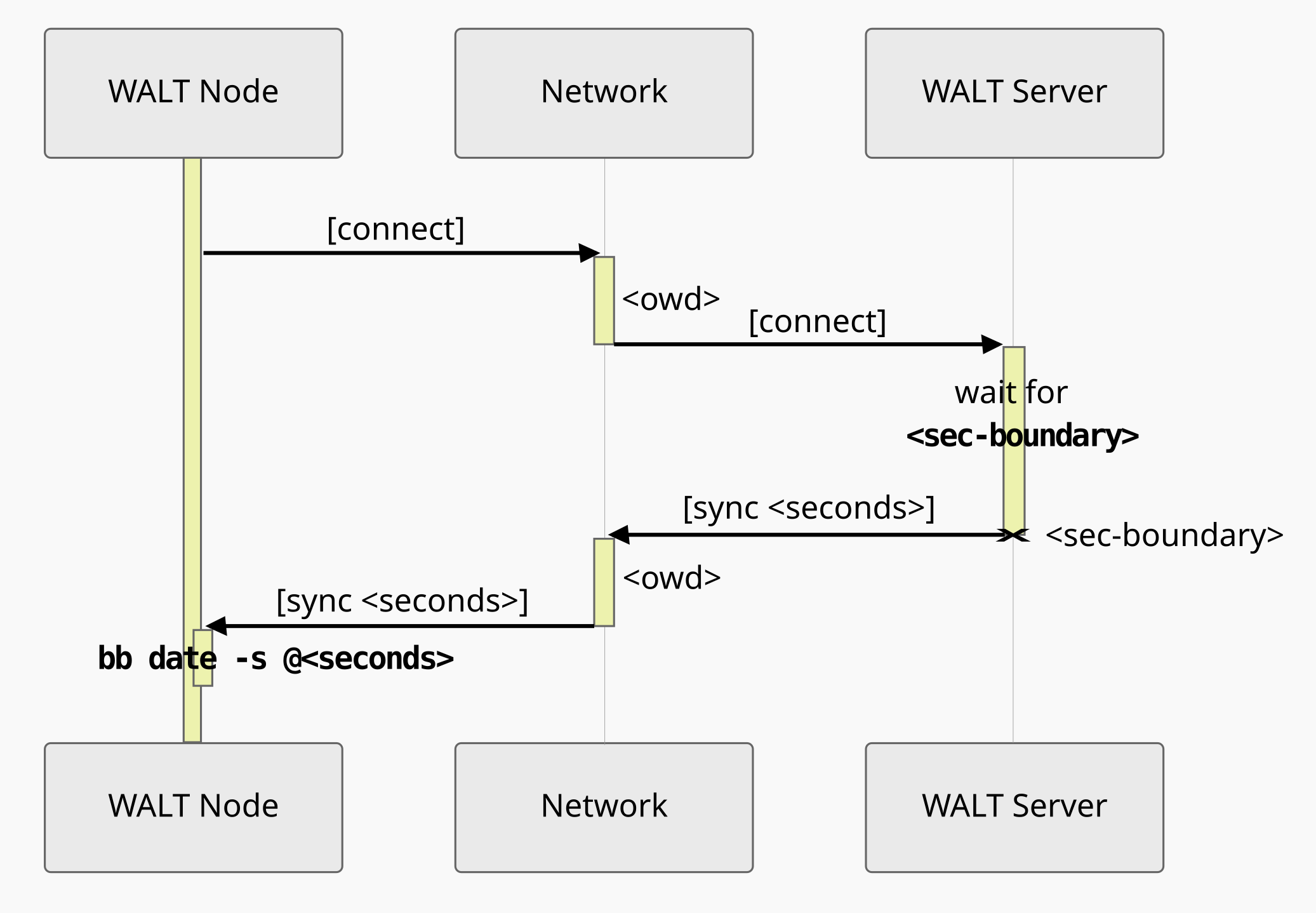
Since busybox date -s <date> only supports setting the date as an integer number of seconds, the server has to wait for the next second boundary (<sec-boundary> on the diagram) before sending the synchronization message.
This basic synchronization has the following flaws:
- It does not take into account the network latency (one-way-delay,
<owd>on the diagram), which can be high in the case of VPN nodes. - The command
busybox date -s <date>cannot be very precise because just launching the binary takes a little time (typically more than 1 millisecond); the nodes’ clocks therefore lag behind the server. - On server side, the python code might be busy with something else and lower the accuracy a little more.
- More importantly, this mechanism is a “one shot” synchronization, and if no NTP or PTP daemon is later started by the OS, the clock will start to drift continuously. A computer clock generally drifts by several milliseconds per hour.
Improving the generic synchronization (WALT version >= 11)
WALT v11 will provide the same three options:
- PTP
- NTP
- Generic synchronization, as a fallback.
However, the generic synchronization will be more precise. Furthermore, if no NTP or PTP daemon is subsequently started by the OS —and provided the busybox binary includes the adjtimex applet— it will continue to run on the node to keep the clock synchronized.1
The following sequence diagram describes the new process:
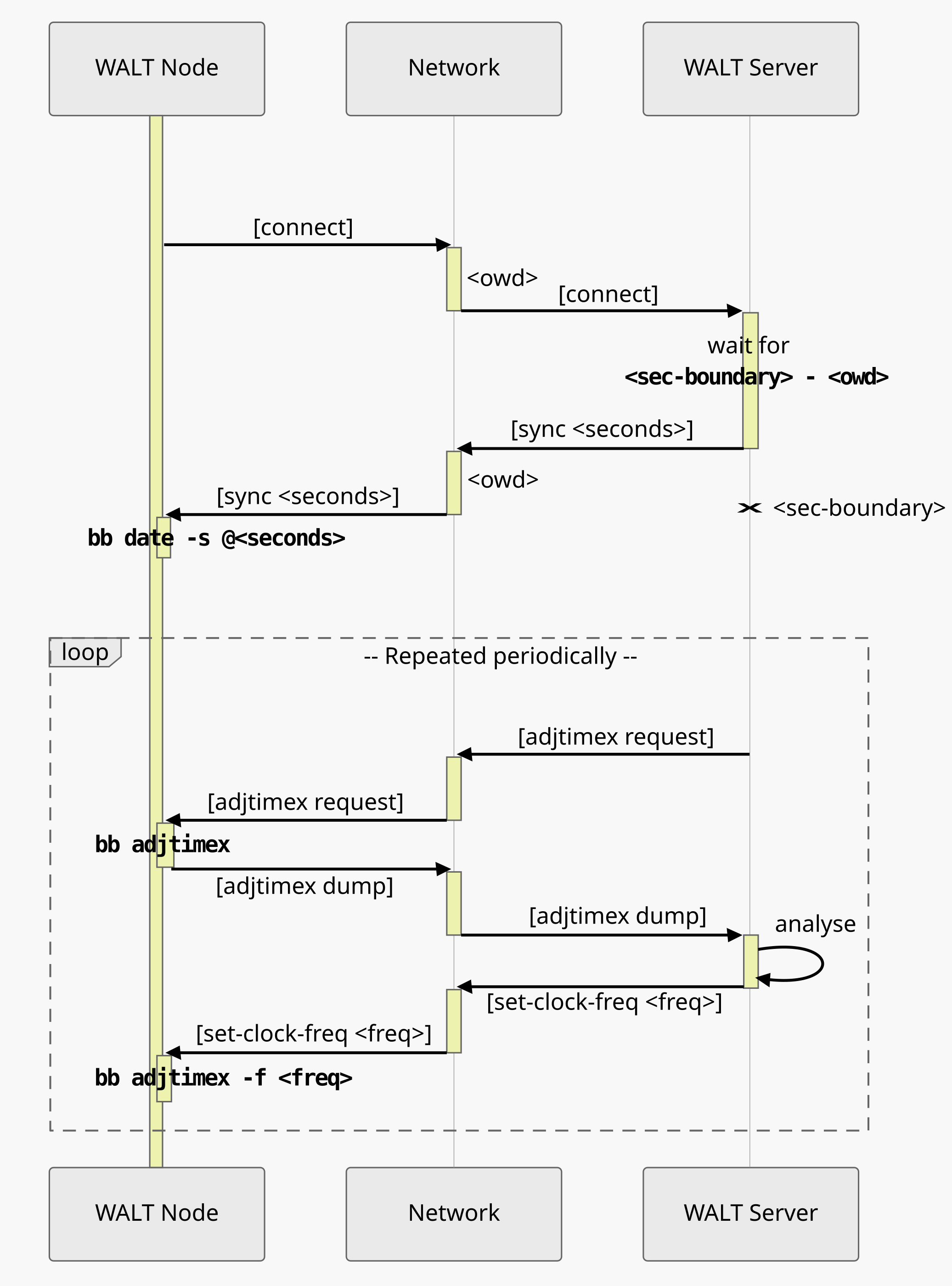
It starts with a first boot-time clock synchronization, similar to what we did previously. But this time, the network latency is taken into account: the server sends the synchronization message a little earlier than the next second boundary so that it is received at the right time2. Moreover, the timestamping on server-side is more accurate than before because this algorithm is now implemented in the C language.
However, the delay for executing busybox date -s @<seconds> on node-side is still there, so the clock of the node probably lags one millisecond or more behind the server after this first phase.
After this first phase, we use another busybox applet called adjtimex to repeatedly adjust the clock frequency: busybox adjtimex -f <freq>. The parameter <freq> is the acceleration or deceleration ratio that should be applied to cancel out the hardware clock drift. In this second phase, since we are acting on the node’s clock frequency rather than the offset, we no longer require high precision regarding the exact moment a change is applied.
Using busybox adjtimex without arguments returns the current adjustment parameters and, crucially, a precise time with fine granularity (down to the microsecond or nanosecond, depending on the kernel).
Since it is hard to run computations fast enough on node-side with the limited busybox-based tooling, at each step of the loop the node just dumps the output of busybox adjtimex on the network connection3 and the analysis is then done on server side.
On the server side, the calculations performed at each step of the loop rely on five timestamps:
t0: server timestamp at the last stepremote_t0: node timestamp at the last stept1: server timestamp at the current step (time when theadjtimexdump was received)remote_t1: node timestamp at the current step (time indicated in theadjtimexdump +<owd>)4t2: server time planned for next step
Let’s also define the following values:
δ0 = remote_t0 - t0
δ1 = remote_t1 - t1
The following diagram allows to visualize how we will proceed.
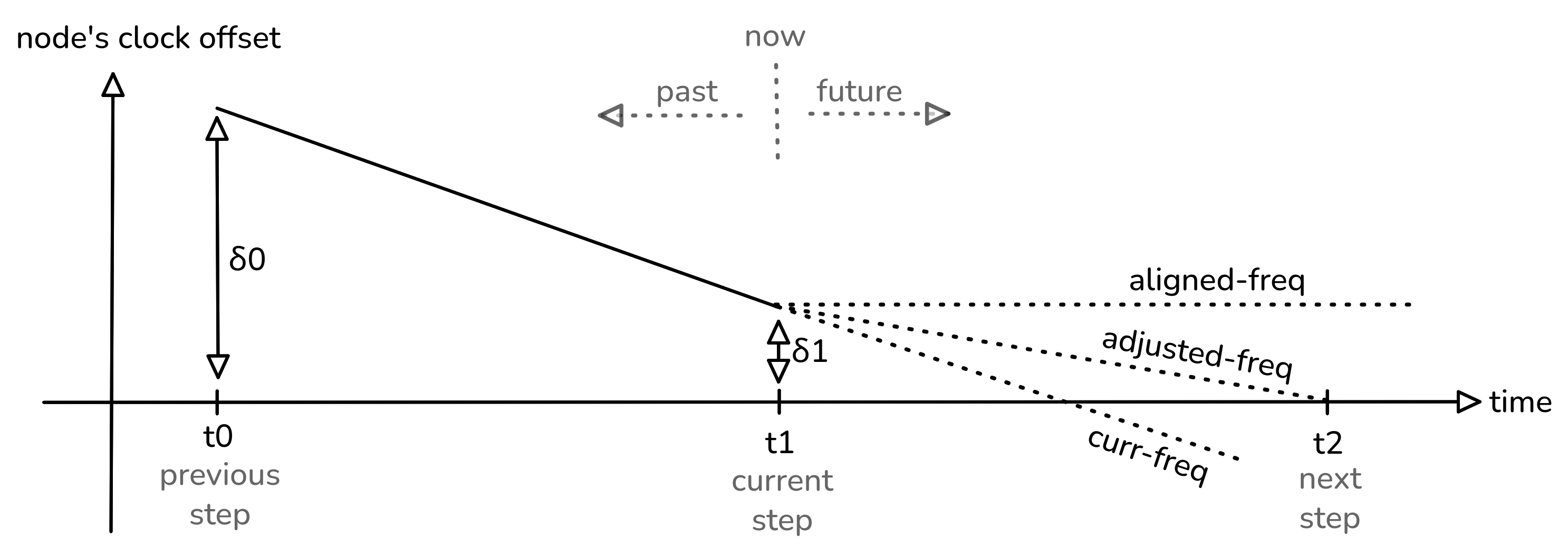
Our goal is to assess the value of adjusted-freq allowing to have the node’s clock synchronized (in terms of offset) to the server’s clock at next step t2.
The frequency curr-freq is the estimate of adjusted-freq we made at the previous step (i.e., at t0), and consequently the frequency which was applied between t0 and t1.
The delay corresponding to the period [t0,t1] is obviously t1-t0 according to the clock of the server, whereas it is remote_t1-remote_t0 according to the node’s clock.
Thus if we want to align the node’s clock frequency with that of the server, we should use the following frequency:
<aligned-freq> = <curr-freq> * (t1-t0) / (remote_t1-remote_t0)
But that aligned frequency is just a first step: it would preserve the offset δ1 instead of removing it at t2.
If we want to have the offset zeroed at t2, we will need the node’s clock to run slower than aligned-freq because its value at t1 is remote_t1=t1+δ1 already.
That’s why we use the following adjusted frequency:
<adjusted-freq> = <aligned-freq> * (t2-remote_t1) / (t2-t1)
Obviously, the accuracy of our measurements is not perfect, and we will probably still observe an offset at next loop step (i.e., at t2). However, by applying this algorithm iteratively and reducing inaccuracies using exponential smoothing, we obtain a quite precise synchronization. The following plot shows how the offset5 of four virtual nodes evolves over a duration of one hour. We have a synchronization step every 15 seconds.
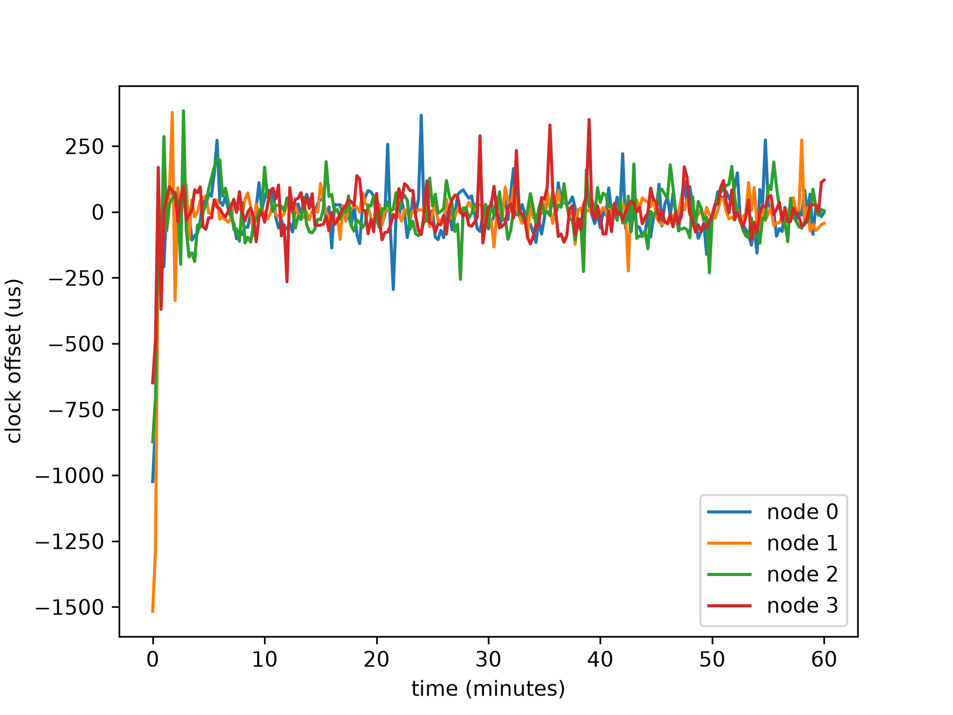
Note that I also tested a Raspberry Pi 5 node and obtained similar results.
After the first sync message, the node’s clock lags around 1 millisecond behind the server clock. But then the clock offset is quickly reduced.
It might be possible to obtain even better accuracy by fine tuning the algorithm parameters, such as the period between two synchronization steps and the smoothing parameters. However, since I was pretty happy with this sub-millisecond accuracy, and for other reasons too6, I stopped here. But obviously, I would welcome any contribution on this!
For the record, I configured one of the four nodes with a round-trip-time value of 30ms. The fact that we cannot visually determine which of the four nodes was configured in this way proves that this parameter is correctly managed.
Notes about synchronizing virtual nodes
One could think that the system clock of virtual nodes is the same as the one of the host. I am not sure about other hypervisors, but with qemu, the one used for WALT virtual nodes, that is not the case.
Physical x86 machines have a hardware clock and a battery on their motherboard used to keep the time when the machine is off. But this hardware clock stores an integer number of seconds; consequently, when the OS boots up and reads this value, its system clock is not set precisely.
qemu emulates this hardware clock device. When the value is read, it returns the value of the host’s system time. But again, because of the integer granularity, the time of the virtual machine is initialized with a value lagging up to one second behind the host system time. And after that, if nothing is done, the system clock starts to drift, similarly to a physical machine.
An option to precisely synchronize a virtual machine to the host is to configure a PTP daemon to use a ptp_kvm virtual clock, which maps to the host’s system time. It is possible for WALT users to configure a WALT image for this. However, since this technique is specific to virtual nodes and requires specific support in WALT OS images, I preferred to focus on a more general solution.
Last words
I hope you found this blog post interesting. At least on my side trying to implement a precise algorithm with the very limited tooling on the node side was quite fun!
Thanks to Jérémie Finiel and Charlélie Pignol for proofreading. If you have questions, we can answer you on the mailing list.
-
If the
busyboxbinary does not provide theadjtimexapplet, then the script ends just after the initial synchronization. And if the script detects that another process of the node started to take care of clock synchronization (probably a PTP or NTP service), it stops too. The script detects this case by checking whether theadjtimexparameters have changed since the last time it set them. ↩︎ -
In order to estimate the one-way-delay value, we use the TCP_INFO socket option. Among the fields available (look for
struct tcp_infoin/usr/include/linux/tcp.h), we read the round-trip-time (RTT) estimation of the kernel and divide this value by two (network links are usually symmetric). ↩︎ -
Similarly to
busybox date -s @<seconds>, executingbusybox adjtimexon the node is not instantaneous. But theclock_gettime()call occurs at the very end of the command’s execution, immediately followed by the writing of the findings to the command’s output. This command’s output is then dumped to the network socket with almost no delay because thebusybox nccommand which is managing the connection is already running since the start of the script. After the one-way-delay, we receive this message on server side. Overall, I estimate that this process provides a reasonably accurate value for the node’s clock, with a maximum offset in the order of a few tens of microseconds. ↩︎ -
The adjtimex dump needs time to cross the network: the time value it contains was obtained at
t1-owd. So in order to assess the synchronization offset properly, we need to add<owd>to this value. ↩︎ -
We plotted the values of
δ1at each synchronization step; the graph therefore represents the server-side view of the clock offsets. ↩︎ -
If the experiment has high time synchronization constraints, users know that they have other options (i.e., PTP or NTP), so it seemed not very useful to spend more time on tuning parameters. Moreover, it is hard to increase the accuracy because of the limited tooling on the node. And the WALT server relies on the NTP protocol to synchronize its own clock, so the clock against which we are attempting to synchronize is not perfectly stable either. Also note that the achievable precision depends on the equipment as well. For instance, old Raspberry Pi boards had their network chip connected with USB, and that could add much inaccuracy to the timestamping. ↩︎